Curves#
A curve maps x from 0 to 1 onto a value. Use it as a hyperparameter schedule — a warmup
then a cosine decay for temperature — or as any other value that should change over the
course of a run.
Curves are project items (curves/<name>.curve.json) with their own editor.
The shape#
A curve is a list of points and, between each pair, a segment with its own interpolation. So one curve can rise linearly, hold flat, then decay exponentially.
| Interpolation | Shape |
|---|---|
linear |
straight |
step |
hold, then jump at the right edge |
smooth |
smoothstep, flat at both ends |
ease-in, ease-out, ease-in-out |
power curves, shaped by k |
cosine |
a half cosine |
exp |
geometric (falls back to linear if an endpoint is ≤ 0) |
log |
logarithmic, shaped by k |
sigmoid |
logistic, normalised so the endpoints are exact |
spline |
Catmull-Rom through the neighbouring points |
bezier |
a CSS-style cubic with four handles |
expr |
your own equation |
Editing#
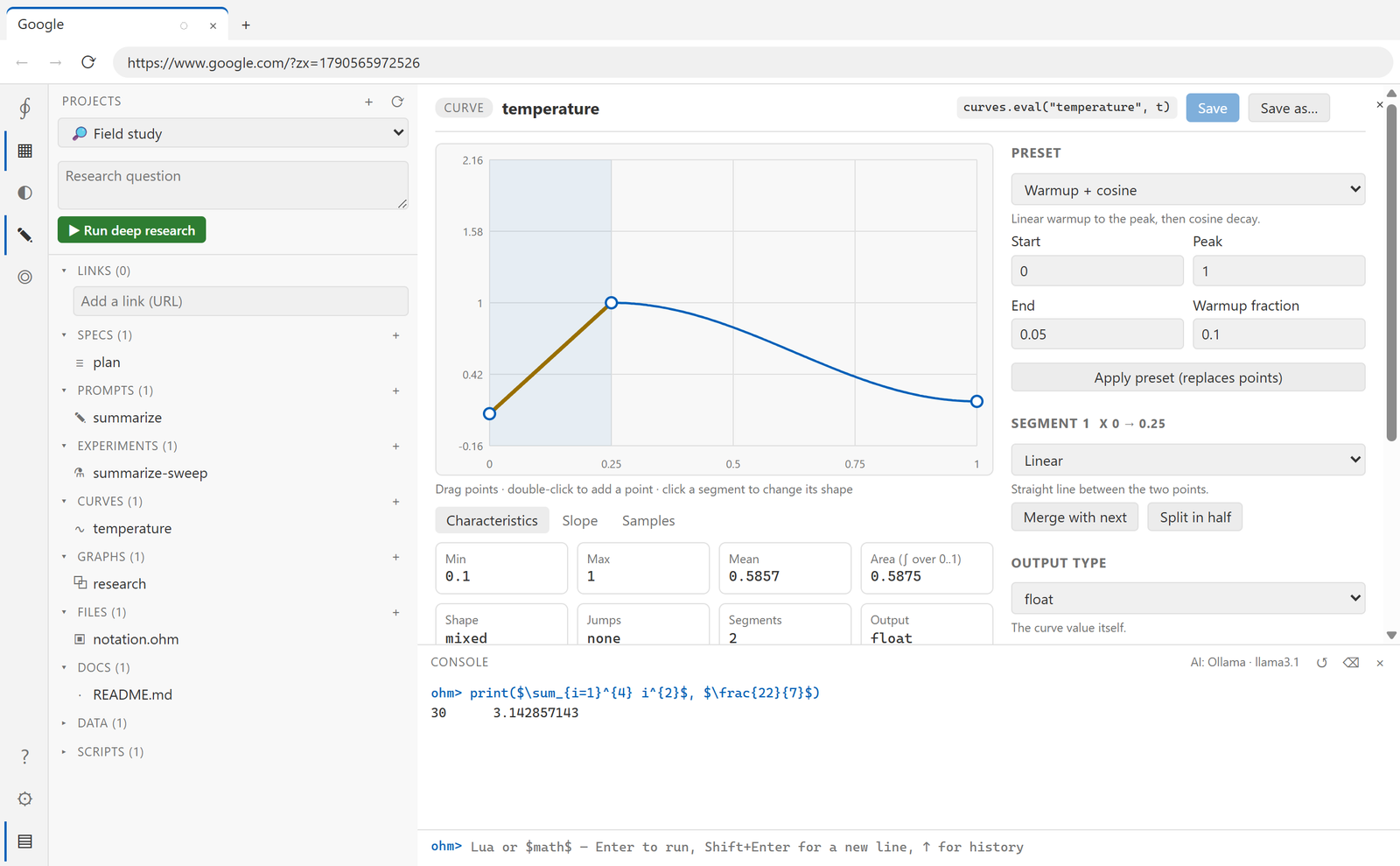
- Drag a point to move it. The first is pinned to x=0 and the last to x=1; interior points stay between their neighbours.
- Double-click the plot to insert a point on the curve.
- Click a segment to select it, then choose its interpolation, split it in half or merge it with the next.
- Presets give you a whole shape at once: constant, linear, cosine, warmup + cosine, exponential decay, step decay, triangular, one-cycle, warm restarts, inverse-sqrt, polynomial, sigmoid — each with its own parameters.
Equations#
Pick expr for a segment and write a formula over u (position within the segment, 0…1),
x (position along the whole curve), y0 and y1 (the segment's endpoints), i (segment
index) and n (segment count):
y1 + (y0 - y1) * (1 - u)^2
y0 / sqrt(1 + 9*u)
lerp(y0, y1, smoothstep(0, 1, u))
Available: sin cos tan asin acos atan atan2 sinh cosh tanh exp log ln log2 log10 sqrt abs sign floor ceil round fract min max pow mod clamp lerp smoothstep step sigmoid, plus pi,
e and tau. Ternaries (c ? a : b) and the usual operators work; ^ is
right-associative.
The expression parser is hand-written — there is no eval — so an equation can only reach
those names. Errors appear live with the character position. A dropdown of ready-made
equations is there to start from.
An equation that fails at runtime quietly returns the segment's left value. If a segment looks flat, check the expression banner.
Typed output#
The raw curve is a number; the output type turns it into what you actually need:
| Type | Result |
|---|---|
float |
the number, optionally rounded to N decimals |
int |
floor, ceil or round |
bool |
true above a threshold (default 0.5) |
enum / string |
the option at that index |
list / set |
the first N options (a set also dedupes) |
Clamps (min/max) apply to the raw value before typing, so they bound the number, not
the option index.
That is how a curve drives a non-numeric setting: a string curve over
["plain", "bullet points", "tweet"] walks a style across an experiment.
Characteristics#
Four tabs under the plot:
- Characteristics — min, max, mean, area under the curve, whether it is monotonic, where it jumps, segment count.
- Slope — the derivative, with a zero line.
- Samples — a table of x, raw value and typed value at N points.
- Value histogram — for non-float outputs, how often each value occurs.
Using a curve#
In an experiment, give a sweep variable the source curve and the curve's
name. In a script:
print(curves.eval("temperature", 0.25))
local xs = curves.sample("temperature", 20)